StateArray
- class StateArray(self, trajectories: TrajectoryGroup, likelihood: :py:class:`Likelihood`, params: StateArrayParameters)
Central class for running state array inference on one SPT experiment. Encapsulates routines to infer the occupation of each point on a parameter grid, given a set of trajectories.
Specifically, suppose that \(\mathbf{X}\) is a set of \(N\) trajectories (using whatever format is most convenient).
We select a grid of \(K\) distinct states (represented, in this case, by the Likelihood object). Each state is associated with some state parameters that define its characteristics. As an example, the RBME likelihood uses two parameters for each state: a diffusion coefficient and a localization error. We use \(\theta_{j}\) to indicate the tuple of all state parameters for state \(j\).
Let \(\mathbf{Z} \in \left\{ 0, 1\right\}^{N \times K}\) be the trajectory-state assignment matrix, so that
\[\begin{split}Z_{ij} = \begin{cases} 1 &\text{if trajectory $i$ is assigned to state $j$} \\ 0 &\text{otherwise} \end{cases}\end{split}\]Further, let \(\boldsymbol{\tau} \in \mathbb{R}^{K}\) be the vector of state occupations, so that \(\sum\limits_{j=1}^{K} \tau_{j} = 1\).
Notice that, given a particular state occupation vector \(\boldsymbol{\tau}\), the probability to see the assignments \(\mathbf{Z}\) is
\[p(\mathbf{Z} | \boldsymbol{\tau}) = \prod\limits_{i=1}^{N} \prod\limits_{j=1}^{K} \tau_{j}^{Z_{ij}}\]Similarly, the probability to see trajectories \(\mathbf{X}\) given the assignment matrix \(\mathbf{Z}\) is
\[p (\mathbf{X} | \mathbf{Z}) = \prod\limits_{i=1}^{N} \prod\limits_{j=1}^{K} f(X_{i}|\theta_{j})^{Z_{ij}}\]where \(f(X_{i}|\theta_{j})\) is the likelihood function for state \(j\) evaluated on trajectory \(i\).
We seek the posterior distribution \(p(\mathbf{Z}, \boldsymbol{\tau} | \mathbf{X})\). The StateArray class uses a variational Bayesian approach that approximates the posterior distribution as the product of two factors:
\[p(\mathbf{Z}, \boldsymbol{\tau} | \mathbf{X}) \approx q(\mathbf{Z}) q(\boldsymbol{\tau})\]The factor \(q(\mathbf{Z})\) is given by the attribute
posterior_assignment_probabilities, while the factor \(q(\boldsymbol{\tau})\) is given by the attributeposterior_occs.For the prior over the trajectory-state assignments, we take a uniform distribution over all states for each trajectory. For the prior over the state occupations, we take:
\[\boldsymbol{\tau} \sim \text{Dirichlet} \left( \alpha \cdot \mathbf{1} \right)\]Here, \(\mathbf{1}\) is a \(K\)-vector of ones and \(\alpha\) is the concentration parameter. Larger values of \(\alpha\) require more data in order to depart from uniformity. The default value of \(\alpha\) (
saspt.constants.DEFAULT_CONC_PARAM) is 1.0. Reasonable values are between 0.5 and 1.0.Additionally, the StateArray object implements an alternative (“naive”) estimator for the state occupations. This is defined as
\[ \begin{align}\begin{aligned}\tau_{j} \propto \eta_{j}^{-1} \sum\limits_{i=1}^{N} n_{i} r_{ij}\\r_{ij} = \frac{ f(X_{i}|\theta_{j}) }{ \sum\limits_{k=1}^{K} f(X_{i}|\theta_{k})}\end{aligned}\end{align} \]where \(n_{i}\) is the number of jumps in trajectory \(i\) and \(\eta_{j}\) is a correction for defocalization of state \(j\). The naive estimator is considerably less precise than the posterior occupations, but has the virtue of speed and simplicity.
- Parameters
trajectories (TrajectoryGroup) – a set of trajectories to run this state array on
likelihood (Likelihood) – the likelihood function to use
params (StateArrayParameters) – parameters governing the state array algorithm, including the concentration parameter, maximum number of iterations, and so on
- likelihood: Likelihood
The underlying likelihood function for this StateArray
- trajectories: TrajectoryGroup
The underlying set of trajectories for this StateArray
- classmethod from_detections(cls, detections: pandas.DataFrame, likelihood_type: str, **kwargs)
Alternative constructor; make a StateArray directly from a set of detections. This avoids the user needing to explicitly construct the Likelihood and StateArrayParameters objects.
- Parameters
detections (pandas.DataFrame) – input set of detections, with the columns frame (
saspt.constants.FRAME), trajectory (saspt.constants.TRACK), y (saspt.constants.PY), and x (saspt.constants.PX)likelihood_type (str) – the type of likelihood function to use; an element of saspt.constants.LIKELIHOOD_TYPES
kwargs – additional keyword arguments to the StateArrayParameters and Likelihood subclass. Must include pixel_size_um and frame_interval.
- Returns
new instance of StateArray
- property n_tracks: int
Number of trajectories in this SPT experiment after preprocessing. See TrajectoryGroup.
- property n_jumps: int
Number of jumps (particle-particle links) in this SPT experiment after preprocessing. See TrajectoryGroup.
- property n_detections: int
Number of detections in this SPT experiment after preprocessing. See TrajectoryGroup.
- property shape: Tuple[int]
Shape of the parameter grid on which this state array is defined. Alias for StateArray.likelihood.shape.
- property likelihood_type: str
Name of the likelihood function. Alias for StateArray.likelihood.name.
- property parameter_names: Tuple[str]
Names of the parameters corresponding to each axis in the parameter grid. Alias for StateArray.likelihood.parameter_names
- property parameter_values: Tuple[numpy.ndarray]
Values of the parameters corresponding to each axis in the parameter grid. Alias for StateArray.likelihood.parameter_values.
- property n_states: int
Total number of states in the parameter grid; equivalent to the product of the dimensions of the parameter grid
- property jumps_per_track: numpy.ndarray
1D numpy.ndarray of shape (n_tracks,); number of jumps in each trajectory
- property naive_assignment_probabilities: numpy.ndarray
numpy.ndarray of shape (*self.shape, n_tracks); the “naive” probabilities for each trajectory-state assignment. These are just normalized likelihoods, and provide a useful counterpoint to the posterior trajectory-state assignments.
The naive probability to assign trajectory \(i\) to state \(j\) in a model with \(K\) total states is
\[r_{ij} = \frac{ f(X_{i}|\theta_{j}) }{ \sum\limits_{k=1}^{K} f(X_{i}|\theta_{k})}\]where \(f(X_{i}|\theta_{j})\) is the likelihood function evaluated on trajectory \(X_{i}\) with state parameter(s) \(\theta_{j}\).
Example:
>>> from saspt import sample_detections, StateArray, RBME

# Make a StateArray
>>> SA = StateArray.from_detections(
...     sample_detections(),
...     likelihood_type = RBME,
...     pixel_size_um = 0.16,
...     frame_interval = 0.00748
... )
>>> print(f"Shape of parameter grid: {SA.shape}")
Shape of parameter grid: (101, 36)

>>> print(f"Number of trajectories: {SA.n_tracks}")
Number of trajectories: 64

# Get the probabilities for each trajectory-state assignment
>>> naive_assign_probs = SA.naive_assignment_probabilities
>>> print(f"Shape of assignment probability matrix: {naive_assign_probs.shape}")
Shape of assignment probability matrix: (101, 36, 64)

# Example: probability to assign trajectory 10 to state (0, 24)
>>> p = naive_assign_probs[0, 24, 10]
>>> print(f"Naive probability to assign track 10 to state (0, 24): {p}")
Naive probability to assign track 10 to state (0, 24): 0.0018974905182505026

# Assignment probabilities are normalized over all states for each track
>>> print(naive_assign_probs.sum(axis=(0,1)))
[1. 1. 1. ... 1. 1. 1.]
- property posterior_assignment_probabilities: numpy.ndarray
numpy.ndarray of shape (*self.shape, n_tracks); the posterior probabilities for each trajectory-state assignment.
In math, if we have \(N\) trajectories and \(K\) states, then the posterior distribution over trajectory-state assignments is
\[p(\mathbf{Z} | \mathbf{r}) = \prod\limits_{i=1}^{N} \prod\limits_{j=1}^{K} r_{ij}^{Z_{ij}}\]where \(\mathbf{Z} \in \left\{ 0, 1 \right\}^{N \times K}\) is a matrix of trajectory-state assignments and \(\mathbf{r} \in \mathbb{R}^{N \times K}\) is
posterior_assignment_probabilities.The distribution is normalized over all trajectories: \(\sum\limits_{j=1}^{K} r_{ij} = 1\) for any \(i\).
- property prior_dirichlet_param: numpy.ndarray
Shape self.shape; the parameter to the Dirichlet prior distribution over state occupations.
saSPT uses uniform priors by default.
In math:
\[\boldsymbol{\tau} \sim \text{Dirichlet} \left( \boldsymbol{\alpha}_{0} \right)\]where \(\boldsymbol{\tau}\) are the state occupations and \(\boldsymbol{\alpha}_{0}\) is
prior_dirichlet_param.
- property posterior_dirichlet_param: numpy.ndarray
Shape self.shape; the parameter to the Dirichlet posterior distribution over state occupations.
In math:
\[\boldsymbol{\tau} \: | \: \mathbf{X} \sim \text{Dirichlet} \left( \boldsymbol{\alpha} + \boldsymbol{\alpha}_{0} \right)\]where \(\boldsymbol{\tau}\) are the state occupations, \(\boldsymbol{\alpha}\) is
posterior_dirichlet_param, and \(\boldsymbol{\alpha}_{0}\) isprior_dirichlet_param.
- property prior_occs: numpy.ndarray
Shape self.shape; mean occupations of each state in the parameter grid under the prior distribution. Since saSPT uses uniform priors, all values are equal to
1.0/self.n_states(\(1/K\)).\[\boldsymbol{\tau}^{\text{(prior)}} = \mathbb{E} \left[ \boldsymbol{\tau} \right] = \int \boldsymbol{\tau} \: p(\boldsymbol{\tau}) \: d \boldsymbol{\tau} = \frac{1}{K}\]where \(p(\boldsymbol{\tau})\) is the prior distribution over the state occupations and \(K\) is the number of states.
- property naive_occs: numpy.ndarray
Shape self.shape; naive estimate for the occupations of each state in the parameter grid.
These are obtained from the naive trajectory-state assignment probabilities by normalizing a weighted sum across all trajectories:
\[\tau^{\text{(naive)}}_{j} \propto \eta_{j}^{-1} \sum\limits_{i=1}^{N} n_{i} r_{ij}\]where \(n_{i}\) is the number of jumps in trajectory \(i\), \(r_{ij}\) is the naive probability to assign trajectory \(i\) to state \(j\), and \(\eta_{j}\) is a potential correction factor for defocalization.
The naive state occupations are less precise than the posterior occupations, but also require fewer trajectories to estimate. As a result, they provide a useful “quick and dirty” estimate for state occupations, and also a sanity check when comparing against the posterior occupations.
- property posterior_occs: numpy.ndarray
Shape self.shape; mean occupations of each state in the parameter grid under the posterior distribution:
\[\boldsymbol{\tau}^{\text{(posterior)}} = \mathbb{E} \left[ \boldsymbol{\tau} | \mathbf{X} \right] = \int \boldsymbol{\tau} \: p (\boldsymbol{\tau} | \mathbf{X}) \: d \boldsymbol{\tau}\]
- property posterior_occs_dataframe: pandas.DataFrame
Representation of posterior_occs as a pandas.DataFrame. Each row corresponds to a single state (element in the parameter grid), and the columns include the parameter values, naive occupation, and posterior occupation of that state.
Example:
>>> from saspt import sample_detections, StateArray, RBME

# Make a toy StateArray
>>> SA = StateArray.from_detections(sample_detections(),
...     likelihood_type=RBME, pixel_size_um = 0.16,
...     frame_interval = 0.00748, focal_depth = 0.7)

# Get the posterior distribution as a pandas.DataFrame
>>> posterior_df = SA.posterior_occs_dataframe
>>> print(posterior_df)

      diff_coef  loc_error  naive_occupation  mean_posterior_occupation
0          0.01      0.000          0.000002                   0.000002
1          0.01      0.002          0.000003                   0.000002
2          0.01      0.004          0.000004                   0.000003
3          0.01      0.006          0.000005                   0.000004
4          0.01      0.008          0.000009                   0.000007
...         ...        ...               ...                        ...
3631     100.00      0.062          0.000007                   0.000007
3632     100.00      0.064          0.000007                   0.000007
3633     100.00      0.066          0.000007                   0.000007
3634     100.00      0.068          0.000007                   0.000007
3635     100.00      0.070          0.000007                   0.000007
As an example calculation, we can estimate the fraction of particles with diffusion coefficients in the range 1.0 to 10.0 µm2/sec under the posterior distribution:
>>> diff_coefs_in_range = np.logical_and(
...     posterior_diff['diff_coef'] >= 1.0,
...     posterior_diff['diff_coef'] < 10.0)
>>> x = posterior_df.loc[diff_coefs_in_range, 'mean_posterior_occupation'].sum()
>>> print(f"Fraction of particles with diffusion coefficients between 0 and 10: {x}")
0.15984985148415815
And just for fun, we can compare this with the estimate from the naive occupations:
>>> x = posterior_df.loc[diff_coefs_in_range, 'naive_occupation'].sum()
>>> print(f"Fraction of particles with diffusion coefficients between 0 and 10: {x}")
0.15884454681112886
In this case, the naive and posterior estimates agree quite closely. We could get exactly the same result by doing
>>> in_range = np.logical_and(SA.diff_coefs>=1.0, SA.diff_coefs<10.0)

# Fraction of particles with diffusion coefficients in this range,
# under posterior mean occupations
>>> print(SA.posterior_occs[in_range,:].sum())
0.15984985148415815

# Fraction of particles with diffusion coefficients in this range,
# under the naive occupations
>>> print(SA.naive_occs[in_range,:].sum())
0.15884454681112886
- property diff_coefs: numpy.ndarray
1D numpy.ndarray, the set of diffusion coefficients on which this state array is defined, corresponding to one of the axes in the parameter grid.
Not all likelihood functions may use diffusion coefficient as a parameter. In those cases, diff_coefs is an empty numpy.ndarray.
- marginalize_on_diff_coef:
Alias for Likelihood.marginalize_on_diff_coef.
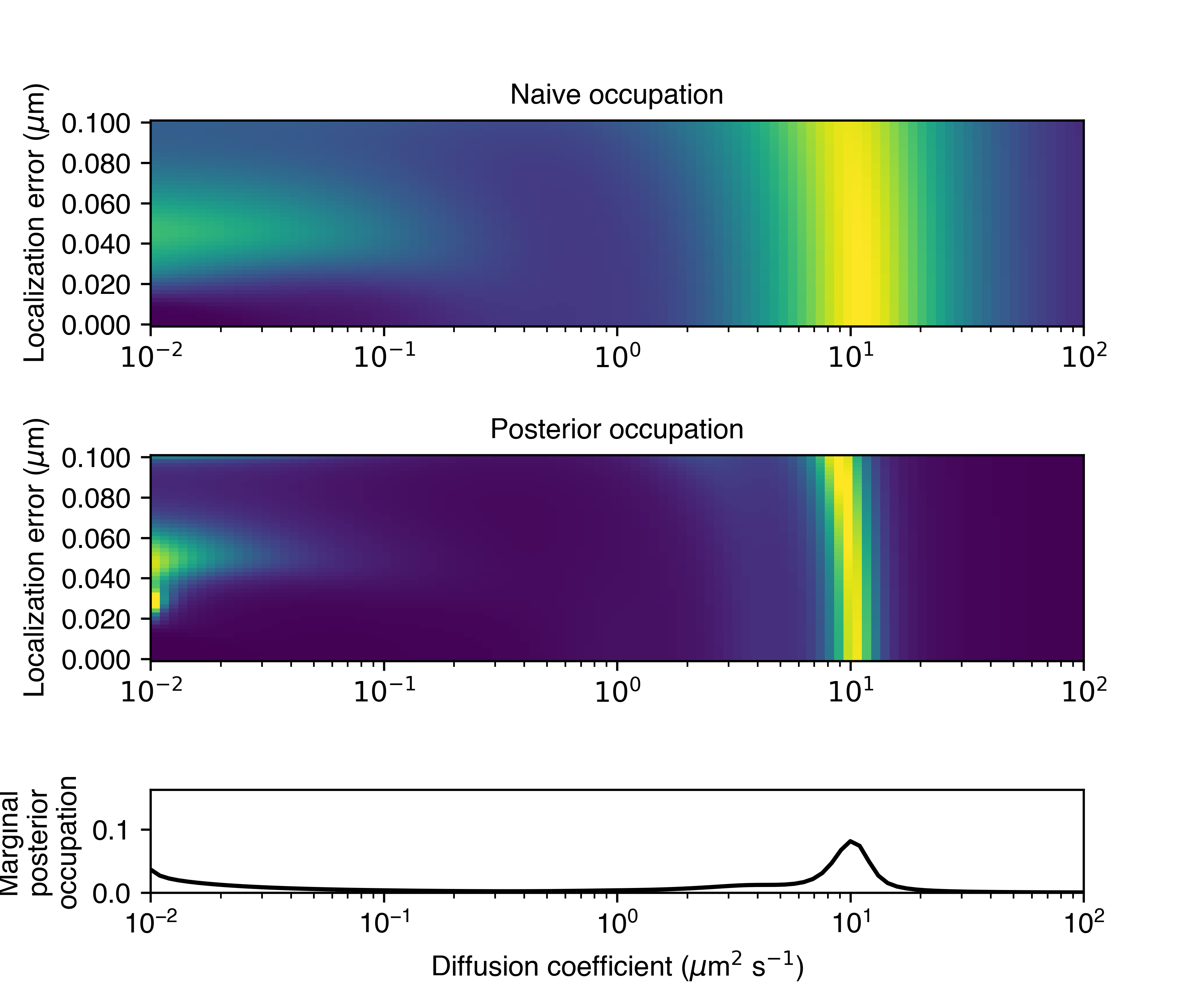
- plot_occupations(self, out_png: str, **kwargs)
Plot the naive and posterior occupations. The exact plot will depend on
likelihood_type. For the RBME likelihood, three panels are shown:the upper panel shows the naive state occupations
the middle panel shows the posterior state occupations
the lower panel shows the posterior state occupations marginalized on diffusion coefficient
- Parameters
out_png (str) – save path for this plot
kwargs – additional kwargs to the plotting function
- plot_assignment_probabilities(self, out_png: str, **kwargs)
Plot the naive posterior trajectory-state assignments, marginalized on diffusion coefficient. Useful for judging heterogeneity between trajectories.
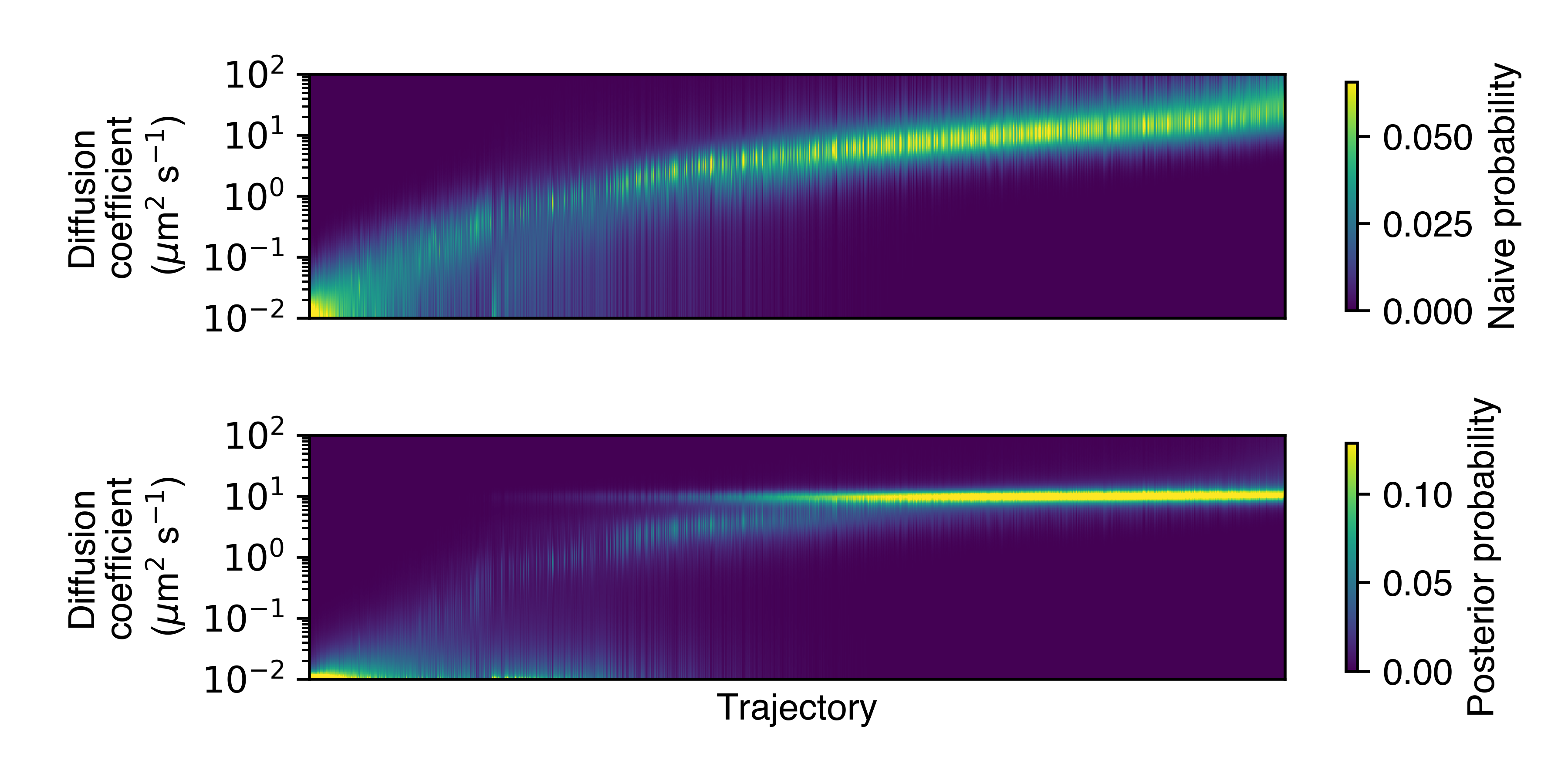
- Parameters
out_png (str) – save path for this plot
kwargs – additional kwargs to the plotting function
- plot_temporal_assignment_probabilities(self, out_png: str, frame_block_size: int = None, **kwargs)
Plot the posterior diffusion coefficient as a function of frame. Useful to judge whether the posterior distribution is stationary. This may not be the case if, for instance, there are lots of tracking errors in the earlier, denser part of the SPT movie.
The color map is proportional to the number of jumps in each frame block by default. To disable this, set the normalize parameter to True.
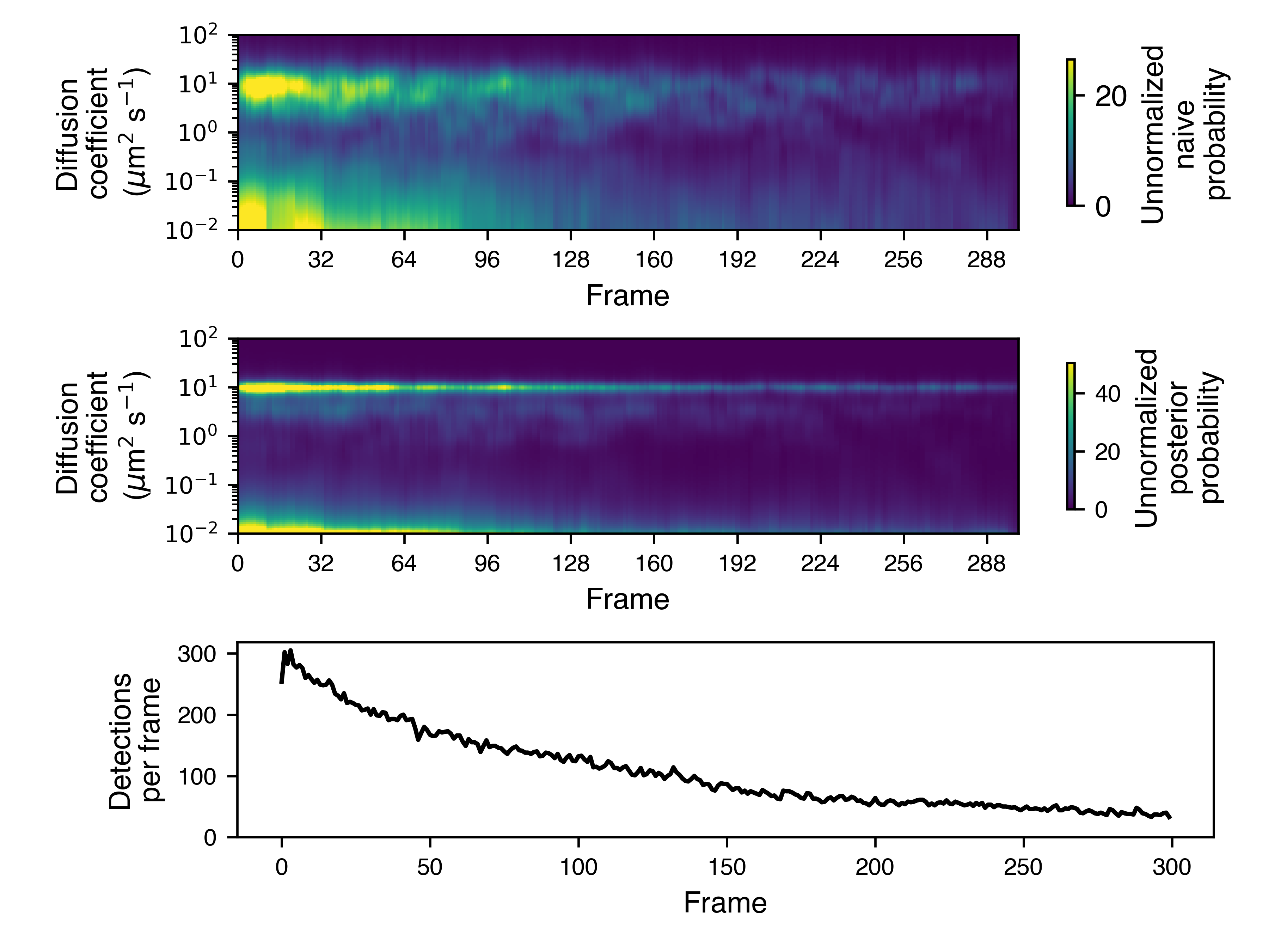
- Parameters
out_png (str) – save path for this plot
frame_block_size (int) – number of frames per temporal bin. If
None, attempts to find an appropriate block size for the SPT movie.kwargs – additional kwargs to the plotting function
- plot_spatial_assignment_probabilities(self, out_png: str, **kwargs)
Plot the mean posterior diffusion coefficient as a function of space. Currently experimental and subject to change.
- Parameters
out_png (str) – save path for this plot
kwargs – additional kwargs to the plotting function