Quickstart
Note
Before running, see Install for installation instructions.
Note
Want more code and less prose? Check out examples.py, a simple executable that demos most of stuff in this Quickstart.
This is a quick guide to getting started with saspt. It assumes you’re familiar
with single particle tracking (SPT), have seen mixture models before, and have
installed saspt.
For a more detailed explanation of saspt’s purpose, model, and range of applicability,
see Background.
Run state arrays on a single SPT experiment
We’ll use the sample set of trajectories that comes with saspt:
>>> import pandas as pd, numpy as np, matplotlib.pyplot as plt
>>> from saspt import sample_detections, StateArray, RBME
>>> detections = sample_detections()
The expected format for input trajectories is described under Note on input format. Importantly, the units for the XY coordinates are in pixels, not microns.
Next, we’ll set the parameters for a state array that uses mixtures of regular Brownian motions with localization error (RBMEs):
>>> settings = dict(
...     likelihood_type = RBME,
...     pixel_size_um = 0.122,
...     frame_interval = 0.01,
...     focal_depth = 0.7,
...     progress_bar = True,
... )
Only three parameters are actually required:
likelihood_type: the type of physical model to use
pixel_size_um: size of camera pixels after magnification in microns
frame_interval: time between frames in seconds
Additionally, we’ve set the focal_depth, which accounts for the finite focal depth of
high-NA objectives used for SPT experiments, and progress_bar, which shows progress
during inference. A full list of parameters and their meaning is described at StateArrayParameters.
Construct a StateArray with these settings:
>>> SA = StateArray.from_detections(detections, **settings)
If we run print(SA), we get
StateArray:
  likelihood_type   : rbme
  n_tracks          : 1130
  n_jumps           : 3933
  parameter_names   : ('diff_coef', 'loc_error')
  shape             : (100, 36)
This means that this state array infers occupations on a 2D parameter grid of diffusion coefficient
(diff_coef) and localization error (loc_error), using 1130 trajectories. The shape of the
parameter grid is (100, 36), meaning that the grid uses 100 distinct diffusion coefficients
and 36 distinct localization errors (the default). These define the range of physical models that can be
described with this state array. We can get the values of these parameters using the
StateArray.parameter_values attribute:
>>> diff_coefs, loc_errors = SA.parameter_values
>>> print(diff_coefs.shape)
(100,)
>>> print(loc_errors.shape)
(36,)
The StateArray object provides two estimates of the state occupations at each point on
this parameter grid:
The “naive” estimate, a quick and dirty estimate from the raw likelihood function
The “posterior” estimate, which uses the full state array model
The posterior estimate is more precise than the naive estimate, but also requires more trajectories and time. The more trajectories are present in the input, the more precise the posterior estimate becomes.
The StateArray object provides a built-in plot to compare the naive and posterior
estimates:
>>> SA.plot_occupations("rbme_occupations.png")
The plot will look something like this:
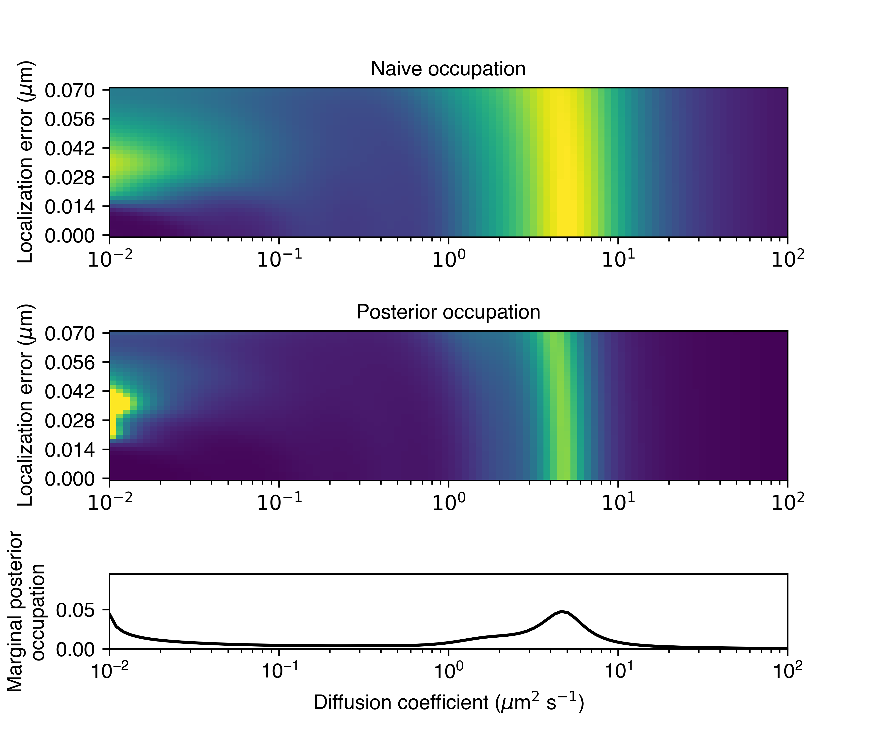
The bottom row shows the posterior occupations marginalized on diffusion coefficient. This is a simple and powerful mechanism to account for the influence of localization error.
In this case, the state array identified a dominant diffusive state with a diffusion coefficient of about 5 \(\mu \text{m}^{2}\)/sec. We can also see a less-populated state between about 1 and 3 \(\mu \text{m}^{2}\)/sec, and some very slow particles with diffusion coefficients in the range 0.01 to 0.1 \(\mu \text{m}^{2}\)/sec.
We can retrieve the raw arrays used in this plot via the naive_occs and posterior_occs
attributes. Both are arrays defined on the same grid of diffusion coefficient vs. localization error:
>>> naive_occs = SA.naive_occs
>>> posterior_occs = SA.posterior_occs
>>> print(naive_occs.shape)
(100, 36)
>>> print(posterior_occs.shape)
(100, 36)
Along with the state occupations, the StateArray object also infers the
probabilities of each trajectory-state assignment. As with the state occupations,
the trajectory-state assignment probabilities have both “naive” and “posterior”
versions that we can compare:
>>> naive_assignment_probabilities = SA.naive_assignment_probabilities
>>> posterior_assignment_probabilities = SA.posterior_assignment_probabilities
>>> print(naive_assignment_probabilities.shape)
(100, 36, 1130)
>>> print(posterior_assignment_probabilities.shape)
(100, 36, 1130)
Notice that these arrays have one element per point in our 100-by-36 parameter grid and per trajectory. For example, the marginal probability that trajectory 100 has each of the 100 diffusion coefficients is:
>>> posterior_assignment_probabilities[:,:,100].sum(axis=1)
StateArray provides a plot to compare the naive and posterior assignment
probabilities across all trajectories:
>>> SA.plot_assignment_probabilities('rbme_assignment_probabilities.png')
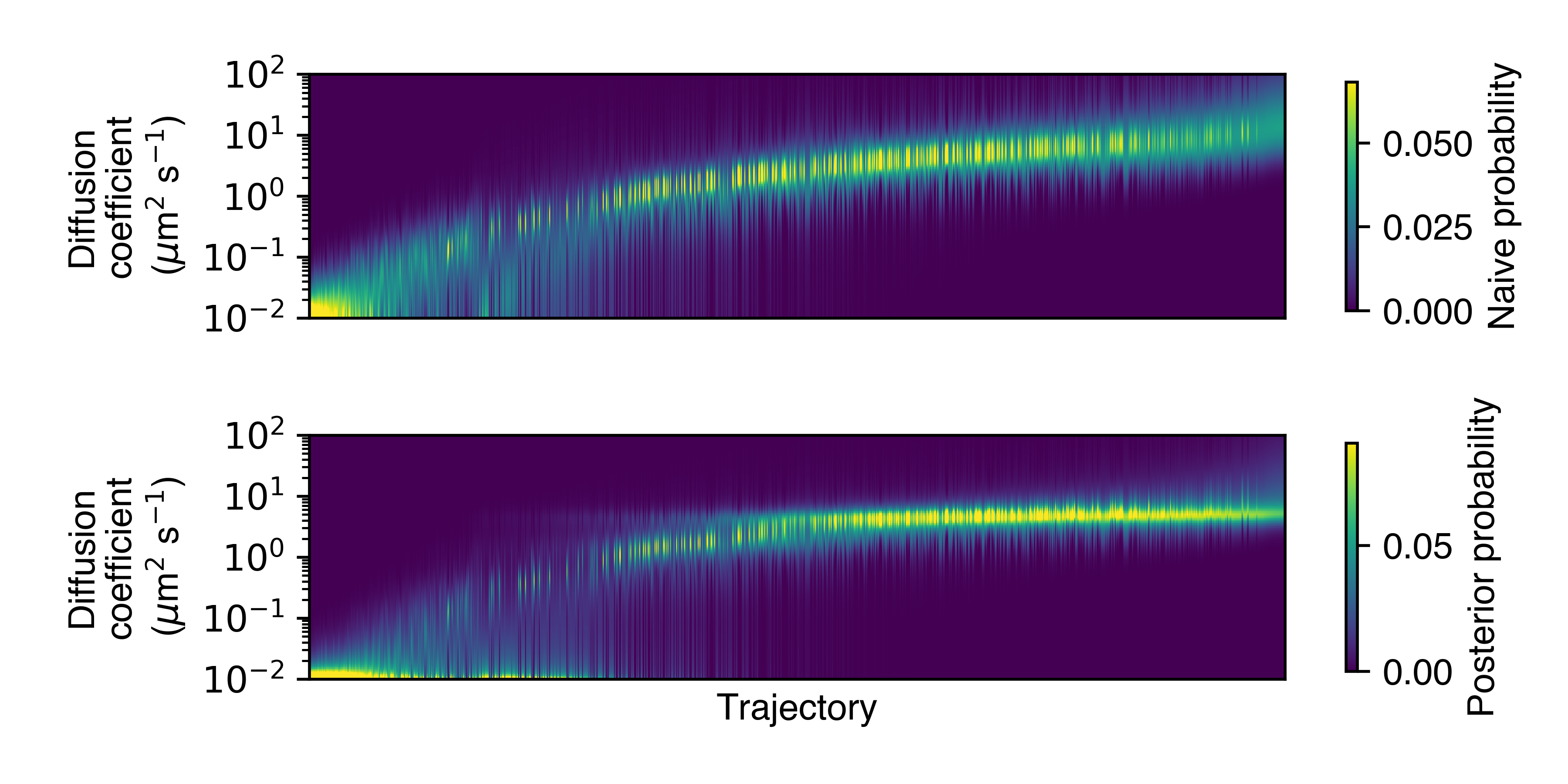
Each column in this plot represents a single trajectory, and the rows represent the probability of the trajectories having a particular diffusion coefficient. (The trajectories are sorted by their posterior mean diffusion coefficient.)
- There are also a couple of related plots (not illustrated here):
saspt.StateArray.plot_temporal_assignment_probabilities(): shows the assignment probabilities as a function of the frame(s) in which the respective trajectories were foundsaspt.StateArray.plot_spatial_assignment_probabilities(): shows the assignment probabilities as a function of the spatial location of the component detections
Finally, StateArray provides the naive and posterior state occupations as a
pandas.DataFrame:
>>> occupations = SA.occupations_dataframe
>>> print(occupations)
      diff_coef  loc_error  naive_occupation  mean_posterior_occupation
0          0.01      0.000          0.000017                   0.000009
1          0.01      0.002          0.000017                   0.000008
2          0.01      0.004          0.000016                   0.000008
...         ...        ...               ...                        ...
3597     100.00      0.066          0.000042                   0.000014
3598     100.00      0.068          0.000041                   0.000014
3599     100.00      0.070          0.000041                   0.000014

[3600 rows x 4 columns]
Each row corresponds to a single point on the parameter grid. For instance, if we wanted to get the probability that a particle has a diffusion coefficient less than 0.1 \(\mu \text{m}^{2}\)/sec, we could do:
>>> selected = occupations['diff_coef'] < 0.1
>>> naive_estimate = occupations.loc[selected, 'naive_occupation'].sum()
>>> posterior_estimate = occupations.loc[selected, 'mean_posterior_occupation'].sum()
>>> print(naive_estimate)
0.24171198737935867
>>> print(posterior_estimate)
0.2779671727562628
In this case, the naive and posterior estimates are quite similar.
Run state arrays on a SPT dataset
Often we want to run state arrays on more than one SPT experiment and compare the
output between experimental conditions. The StateArrayDataset object is intended to
be a simple solution that provides:
methods to parallelize state array inference across multiple SPT experiments
outputs and visualizations to help compare between experimental conditions
In this example, we’ll use an example
from the saspt repo.
You can follow along by cloning the saspt repo and navigating to
the examples subdirectory:
$ git clone https://github.com/alecheckert/saspt.git
$ cd saspt/examples
$ ls -1
examples.py
experiment_conditions.csv
u2os_ht_nls_7.48ms
u2os_rara_ht_7.48ms
- The
examplessubdirectory contains a small SPT dataset where two proteins have been tracked: HT-NLS: HaloTag (HT) fused to a nuclear localization signal (NLS), labeled with the photoactivatable fluorescent dye PA-JFX549RARA-HT: retinoic acid receptor \(\alpha\) (RARA) fused to HaloTag (HT), labeled with the photoactivatable fluorescent dye PA-JFX549
Each protein has 11 SPT experiments, stored as CSV files in the examples/u2os_ht_nls_7.48ms and
examples/u2os_rara_ht_7.48ms subdirectories. We also have a registry file (experiment_conditions.csv) that contains the assignment of each file to an experimental condition:
>>> paths = pd.read_csv('experiment_conditions.csv')
In this case, we have two columns: filepath encodes the path to the CSV corresponding
to each SPT experiment, while condition encodes the experimental condition. (It doesn’t
actually matter what these are named as long as they match the path_col and condition_col
parameters below.)
>>> print(paths)
                                      filepath     condition
0    u2os_ht_nls_7.48ms/region_0_7ms_trajs.csv   HaloTag-NLS
1   u2os_ht_nls_7.48ms/region_10_7ms_trajs.csv   HaloTag-NLS
2    u2os_ht_nls_7.48ms/region_1_7ms_trajs.csv   HaloTag-NLS
..                                         ...           ...
19  u2os_rara_ht_7.48ms/region_7_7ms_trajs.csv  RARA-HaloTag
20  u2os_rara_ht_7.48ms/region_8_7ms_trajs.csv  RARA-HaloTag
21  u2os_rara_ht_7.48ms/region_9_7ms_trajs.csv  RARA-HaloTag

[22 rows x 2 columns]
Specify some parameters related to this analysis:
>>> settings = dict(
...     likelihood_type = RBME,
...     pixel_size_um = 0.16,
...     frame_interval = 0.00748,
...     focal_depth = 0.7,
...     path_col = 'filepath',
...     condition_col = 'condition',
...     progress_bar = True,
...     num_workers = 6,
... )
Warning
The num_workers attribute specifies the number of parallel processes to use when
running inference. Don’t set this higher than the number of CPUs on your computer, or
you’re likely to suffer performance hits.
Create a StateArrayDataset with these settings:
>>> from saspt import StateArrayDataset
>>> SAD = StateArrayDataset.from_kwargs(paths, **settings)
If you do print(SAD), you’ll get some basic info on this dataset:
>>> print(SAD)
StateArrayDataset:
  likelihood_type    : rbme
  shape              : (100, 36)
  n_files            : 22
  path_col           : filepath
  condition_col      : condition
  conditions         : ['HaloTag-NLS' 'RARA-HaloTag']
We can get more detailed information on these experiments (such as the detection density,
mean trajectory length, etc.) by accessing the raw_track_statistics attribute:
>>> stats = SAD.raw_track_statistics
>>> print(stats)
    n_tracks  n_jumps  ...                                    filepath     condition
0       2387     1520  ...   u2os_ht_nls_7.48ms/region_0_7ms_trajs.csv   HaloTag-NLS
1       4966     5341  ...  u2os_ht_nls_7.48ms/region_10_7ms_trajs.csv   HaloTag-NLS
2       3294     2584  ...   u2os_ht_nls_7.48ms/region_1_7ms_trajs.csv   HaloTag-NLS
..       ...      ...  ...                                         ...           ...
19      5418    13129  ...  u2os_rara_ht_7.48ms/region_7_7ms_trajs.csv  RARA-HaloTag
20      9814    26323  ...  u2os_rara_ht_7.48ms/region_8_7ms_trajs.csv  RARA-HaloTag
21      7530    18978  ...  u2os_rara_ht_7.48ms/region_9_7ms_trajs.csv  RARA-HaloTag

[22 rows x 13 columns]
>>> print(stats.columns)
Index(['n_tracks', 'n_jumps', 'n_detections', 'mean_track_length',
       'max_track_length', 'fraction_singlets', 'fraction_unassigned',
       'mean_jumps_per_track', 'mean_detections_per_frame',
       'max_detections_per_frame', 'fraction_of_frames_with_detections',
       'filepath', 'condition'],
      dtype='object')
To get the naive and posterior state occupations for each file in this dataset:
>>> marginal_naive_occs = SAD.marginal_naive_occs
>>> marginal_posterior_occs = SAD.marginal_posterior_occs
>>> print(marginal_naive_occs.shape)
>>> print(marginal_posterior_occs.shape)
Note
It can take a few minutes to compute the posterior occupations for a dataset of
this size. If you need a quick estimate for a test, try reducing the max_iter
or sample_size parameters.
These occupations are “marginal” in the sense that they’ve been marginalized onto the
parameter of interest in most SPT experiments: the diffusion coefficient. (You can
get the original, unmarginalized occupations via the StateArrayDataset.posterior_occs
and StateArrayDataset.naive_occs attributes.)
The same information is also provided as a pandas.DataFrame:
>>> occupations = SAD.marginal_posterior_occs_dataframe
For example, imagine we want to calculate the posterior probability that a particle had a diffusion coefficient less than 0.5 \(\mu\text{m}^{2}\)/sec for each file. We could do this by taking
>>> print(occupations.loc[occupations['diff_coef'] < 0.5].groupby(
...   'filepath')['mean_posterior_occupation'].sum())
filepath
u2os_ht_nls_7.48ms/region_0_7ms_trajs.csv      0.188782
u2os_ht_nls_7.48ms/region_10_7ms_trajs.csv     0.103510
u2os_ht_nls_7.48ms/region_1_7ms_trajs.csv      0.091148
...
u2os_rara_ht_7.48ms/region_7_7ms_trajs.csv     0.579444
u2os_rara_ht_7.48ms/region_8_7ms_trajs.csv     0.553111
u2os_rara_ht_7.48ms/region_9_7ms_trajs.csv     0.650187
Name: posterior_occupation, dtype: float64
The StateArrayDataset provides a few plots to visualize these occupations:
>>> SAD.posterior_heat_map('posterior_heat_map.png')
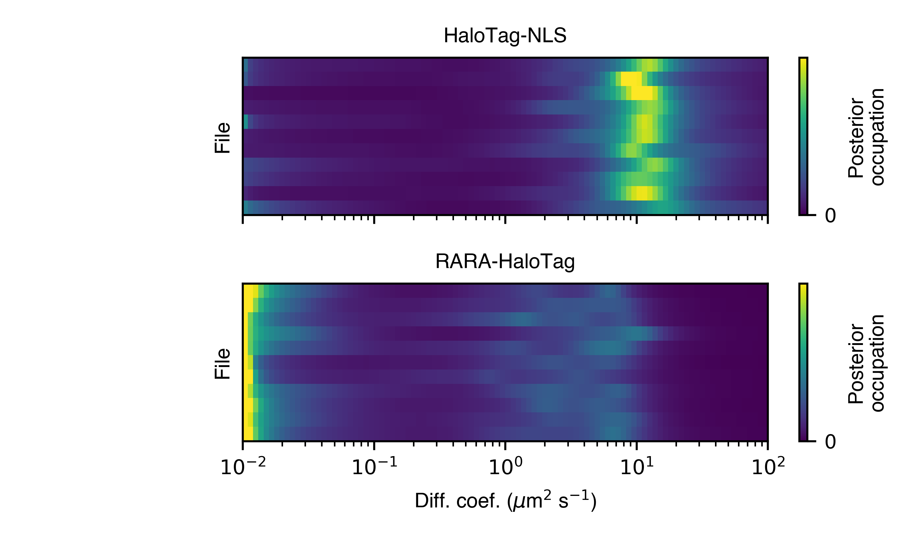
Notice that the two kinds of proteins have different diffusive profiles: HaloTag-NLS occupies a narrow range of diffusion coefficients centered around 10 \(\mu \text{m}^{2}\)/sec, while RARA-HaloTag has a much broader range of free diffusion coefficients with a substantial immobile fraction (showing up at the lower end of the diffusion coefficient range).
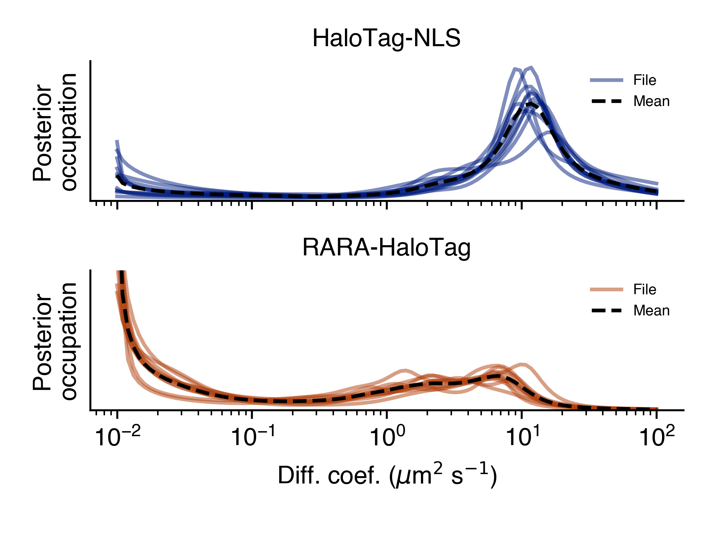
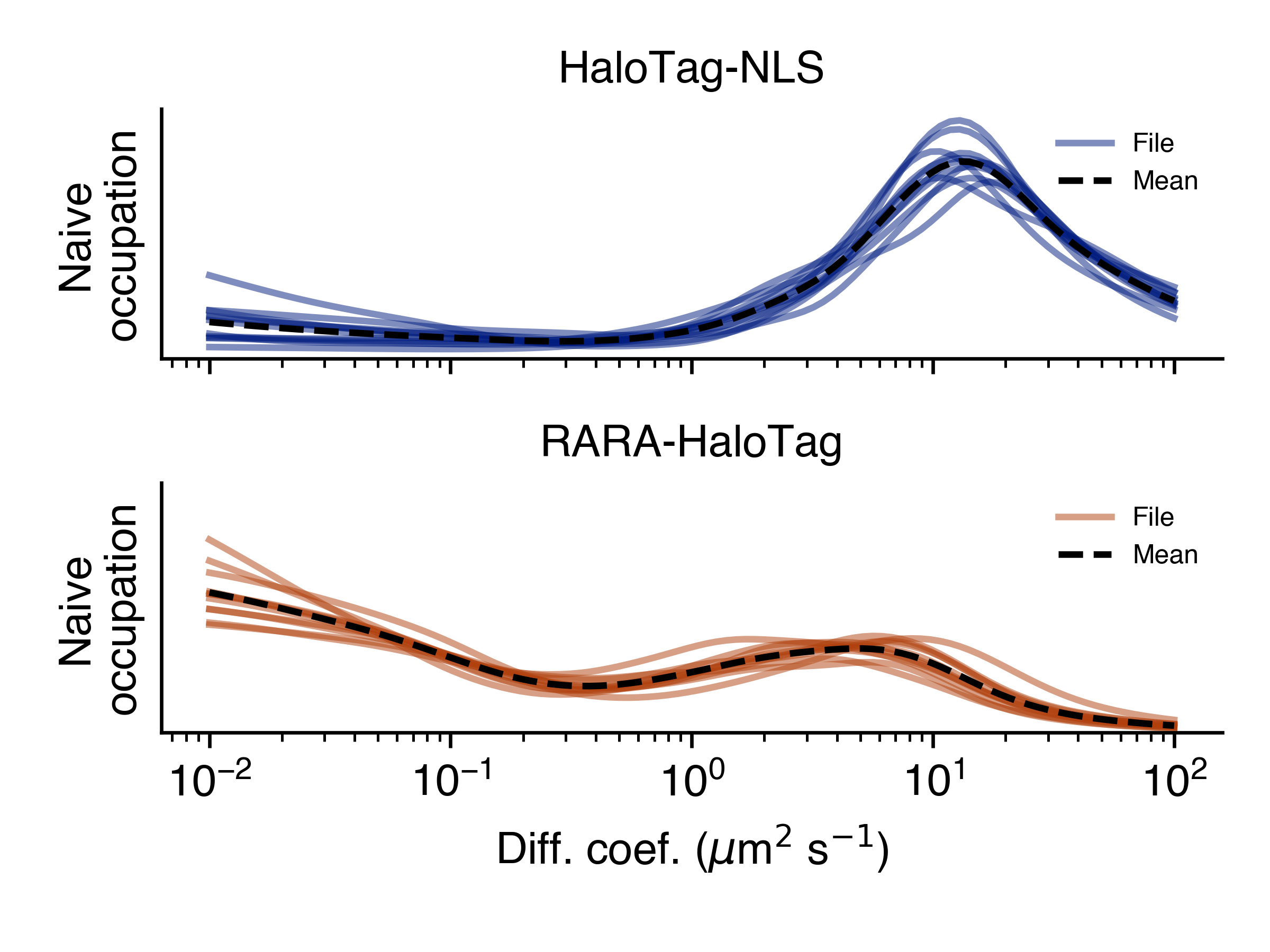
The heat map plot is useful to judge how consistent the result is across SPT experiments in the same condition. We can also compare the variability using an alternative line plot representation:
>>> SAD.posterior_line_plot('posterior_line_plot.png')
>>> SAD.naive_heat_map('naive_heat_map.png')
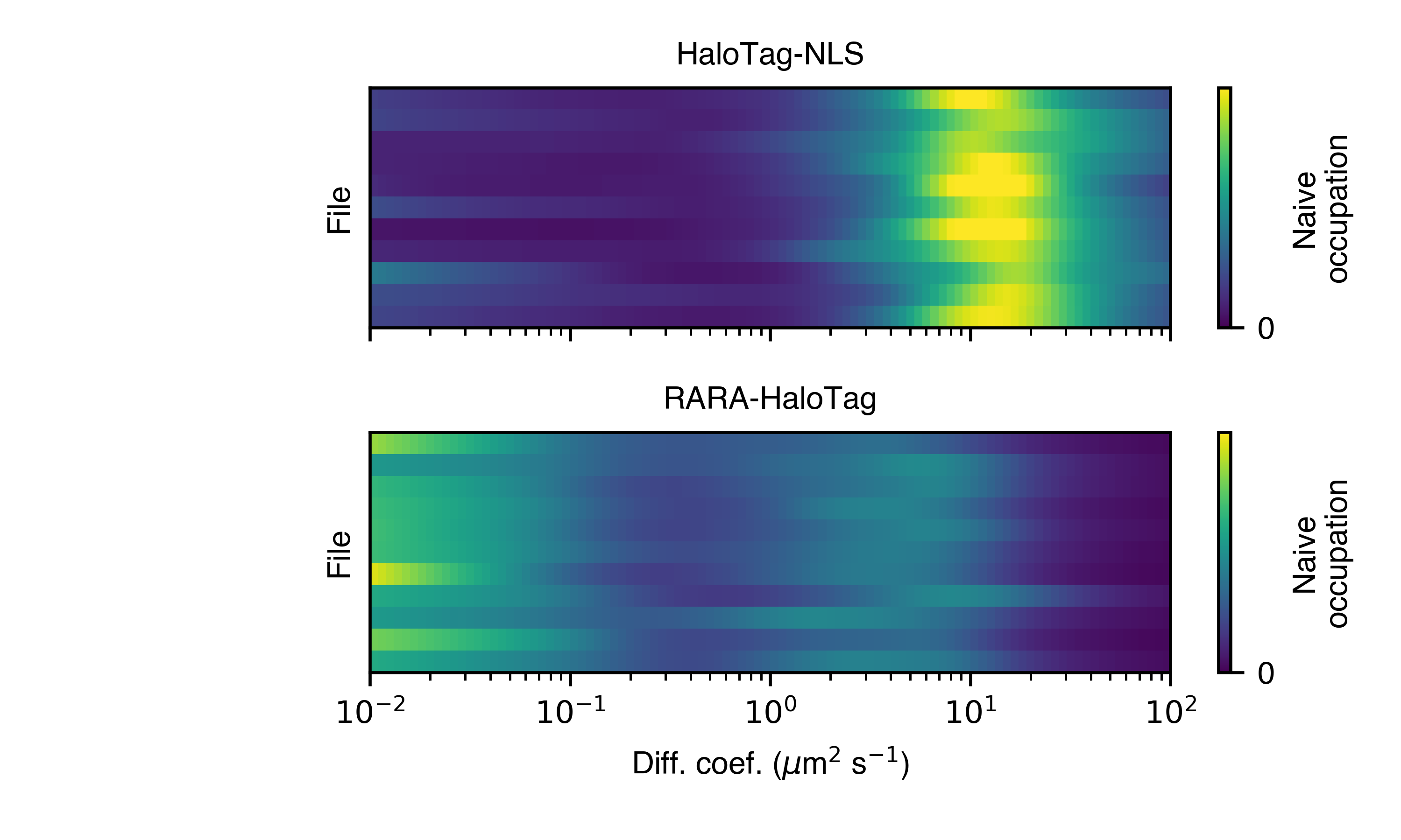
Notice that the information provided by the naive occupations is qualitatively similar but less precise than the posterior occupations.
>>> SAD.naive_line_plot('naive_line_plot.png')
Additionally, rather than performing state array inference on each file individually, we can aggregate trajectories across all files matching a particular condition:
>>> posterior_occs, condition_names = SAD.infer_posterior_by_condition('condition')
>>> print(posterior_occs.shape)
(2, 100)
>>> print(condition_names)
['HaloTag-NLS', 'RARA-HaloTag']
The results are unnormalized (they reflect the total number of jumps in each condition). We can normalize and plot the results by doing:
>>> from saspt import normalize_2d
>>> posterior_occs = normalize_2d(posterior_occs, axis=1)
>>> diff_coefs = SAD.likelihood.diff_coefs
>>> for c in range(posterior_occs.shape[0]):
...     plt.plot(diff_coefs, posterior_occs[c,:], label=condition_names[c])
>>> plt.xscale('log')
>>> plt.xlabel('Diff. coef. ($\mu$m$^{2}$ s$^{-1}$)')
>>> plt.ylabel('Mean posterior occupation')
>>> plt.ylim((0, plt.ylim()[1]))
>>> plt.legend()
>>> plt.show()
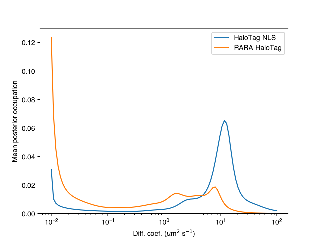
The more trajectories we aggregate, the better our state occupation estimates
become. saspt performs best when using large datasets with tens of thousands of
trajectories per condition.