FAQS

Q. Does saspt provide a way to do tracking?

saspt only analyzes the output of a tracking algorithm; it doesn’t produce the trajectories themselves. The general workflow is:

1. Acquire some raw SPT movies

2. Use a tracking algorithm to produce trajectories from the SPT movie

3. Feed the trajectories into saspt (or whatever your favorite analysis tool is)

There are lots of good tracking algorithms out there. In the sample data included in the saspt repo, we used an in-house tracking tool with a graphic user interface (quot). But - you know - we’re biased.

Other popular options are TrackMate, the multiple-target tracing algorithm, or Sbalzerini’s hill climbing algorithm. There are new tracking algorithms every day; use Google to see for yourself.

Q. Why doesn’t saspt support input format X?

Because a table of detections is probably the simplest format that exists to describe trajectories, so we added it first. We’re happy to expand support for additional formats (within reason) - let us know with a GitHub request.

Q. Why are the default diffusion coefficients log-spaced?

As the diffusion coefficient increases, our estimate of it becomes much more error-prone. This makes it difficult for humans to compare the occupations of states with widely varying diffusion coefficients. By plotting on a log scale, we minimize these perceptual differences so that humans can accurately compare states across the full range of biologically observed diffusion coefficients.

To demonstrate this effect, consider the likelihood function for the jumps of a 2D Brownian motion with no localization error, diffusion coefficient \(D\), frame interval \(\Delta t\), and \(n\) total jumps. The maximum likelihood estimator for the diffusion coefficient is the mean-squared displacement (MSD):

\[\hat{D} = \frac{1}{4 n \Delta t} \sum\limits_{j=1}^{n} (\Delta x_{j}^{2} + \Delta y_{j}^{2})\]

where \((\Delta x_{j}, \Delta y_{j})\) is the \(j^{\text{th}}\) jump in the trajectory.

We can get the “best-case” error in this estimate using the Cramer-Rao lower bound (CRLB), which provides the minimum variance our estimator \(\hat{D}\):

\[\text{Var}(\hat{D}) \geq \text{CRLB}(\hat{D}) = \frac{D^{2}}{n}\]

So the error in the estimate of \(D\) actually increases as the square of \(D\). If we throw in localization error (represented as the 1D spatial measurement variance, \(\sigma^{2}\)) and neglect the off-diagonal terms in the covariance matrix, we get the approximation

\[\text{Var}(\hat{D}) \geq \text{CRLB}(\hat{D}) \approx \frac{(D \Delta t + \sigma^{2})^{2}}{n \Delta t^{2}}\]

Notice that this makes it even harder to estimate the diffusion coefficient, especially when \(D \Delta t < \sigma^{2}\).

Q. How does saspt estimate the posterior occupations, given the posterior distribution?

saspt always uses the posterior mean. If \(\boldsymbol{\alpha}\) is the parameter to the posterior Dirichlet distribution over state occupations, then the posterior mean \(\boldsymbol{\tau}\) is simply the normalized Dirichlet parameter:

\[\begin{split}\boldsymbol{\tau} \sim \text{Dirichlet} \left( \boldsymbol{\alpha} \right) \\ \mathbb{E} \left[ \boldsymbol{\tau} | \boldsymbol{\alpha} \right] = \frac{1}{\sum_{j=1}^{K} \alpha_{j}} \begin{bmatrix} \alpha_{1} \\ ... \\ \alpha_{K} \end{bmatrix}\end{split}\]

We prefer the posterior mean to max a posteriori (MAP) or other estimators because it is very conservative and minimizes the occurrence of spurious features.

Q. I want to measure the fraction of particles in a particular state. How do I do that?

If you know the range of diffusion coefficients you’re interested in, you can directly integrate the mean posterior occupations. Say we want the fraction of particles with diffusion coefficients between 1 and 10 \(\mu\text{m}^{2}\)/sec:

>>> occupations = SA.posterior_occs_dataframe
>>> in_range = (occupations['diff_coef'] >= 1.0) & (occupations['diff_coef'] < 10.0)
>>> print(occupations.loc[in_range, 'mean_posterior_occupation'].sum())

That being said, saspt does not provide any way to determine the endpoints for this range, and that is up to you or the methods you develop.

Q. What is defocalization?

Examining the movie in the section Background, you may notice that the particles are constantly wandering into and out of focus. The faster they move, the faster they escape the microscope’s focus.

As it turns out, this behavior (termed “defocalization”) has a dangerous side effect. If we want to know the state occupations - the fraction of proteins in a particular state - we may be tempted to report the fraction of observed trajectories in that state. The problem is that particles in fast states contribute many short trajectories, because they can wander in and out of focus multiple times before bleaching. By contrast, particles in slow states produce a few long trajectories; they don’t move fast enough to reenter the focal volume before bleaching.

As a result, a mixture of equal parts fast and slow particles does not produce equal parts fast and slow trajectories.

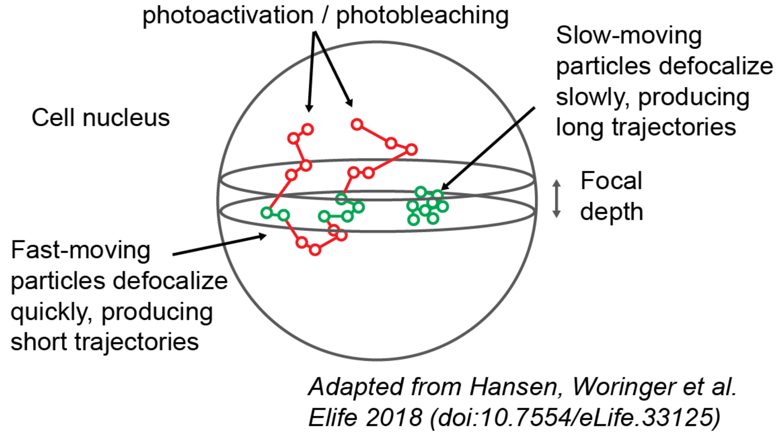
Illustration of the defocalization problem. Particles inside the focus (green circles) are recorded by the microscope; particles outside the focus (red circles) are not recorded. Particles that traverse the focus multiple times are “fragmented” into multiple short trajectories.

Defocalization is the reason why the “MSD histogram” method - one of the most popular approaches to analyze protein tracking data - yields inaccurate results when applied to 2D imaging. A more detailed discussion can be found in the papers of Mazza and Hansen and Woringer.

saspt avoids the state estimation problem by computing state occupations in terms of jumps rather than trajectories. Additionally, an analytical correction factor (analogous to the empirical correction factor from Hansen and Woringer) can be applied to the data by passing the focal_depth parameter when constructing a StateArray or StateArrayDataset object.