The state array model
This section describes the underlying state array model used by saspt. State arrays
are just Bayesian mixture models with large number of mixture components (“states”) that are situated
on a fixed grid of parameters. They rely on a variational Bayesian inference routine that prunes away
superfluous states, selecting minimal models to describe observed SPT datasets.
What makes them work is similar to what makes nonparametric Bayesian
methods work (namely, automatic relevance determination). But their structure leads to a much more efficient and scalable inference routine.
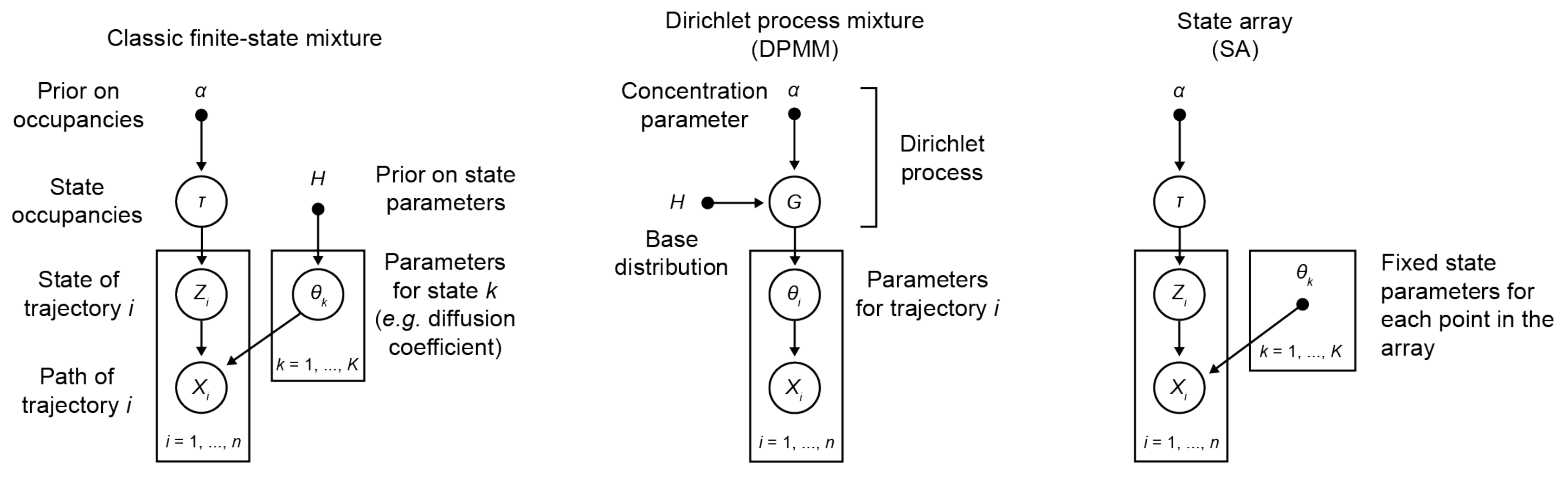
Graphical model comparison of finite state mixtures, Dirichlet process mixtures, and state arrays. Open circles indicate unobserved variables, closed circles/dots indicate observed variables.
Likelihood functions
A physical model for the motion of particles in an SPT experiment is usually expressed in the form of a probability distribution \(p(X|\boldsymbol{\theta})\), where \(X\) is the observed path of the trajectory and \(\boldsymbol{\theta}\) represents the parameters of the motion. Intuitively, this function tells us how likely we are to see a specific trajectory given some kind of physical model. We refer to the function \(p(X|\boldsymbol{\theta})\) as a likelihood function.
As an example, take the case of regular Brownian motion (RBM), a model with a single parameter that characterizes each trajectory (the diffusion coefficient \(D\)). (For those familiar, this is equivalent to a scaled Wiener process.) Its likelihood function is
where \(\Delta r_{k}\) is the radial displacement of the \(k^{\text{th}}\) jump in the trajectory, \(\Delta t\) is the measurement interval, \(d\) is the spatial dimension, and \(n\) is the total number of jumps in the trajectory.
A common approach to recover the parameters of the motion is simply to find the parameters that maximize \(p(X | \boldsymbol{\theta})\), holding \(X\) constant at its observed value. In the case of RBM, this maximum likelihood estimate has a closed form - the mean squared displacement, or “MSD”:
While this works well enough for one pure Brownian trajectory, this approach has several shortcomings when we try to generalize it:
Closed-form maximum likelihood solutions only exist for the simplest physical models, like RBM. Even introducing measurement error, a ubiquitous feature of SPT-PALM experiments, is sufficient to eliminate any closed-form solution.
Maximum likelihood does not provide any measure of confidence in the result. This becomes problematic for complex models with multiple parameters, where a large range of parameter vectors may give near-equivalent results. This means that even when our maximum likelihood estimators work perfectly, they are highly instable from one experiment to the next.
An alternative to maximum likelihood inference is to treat both
\(\mathbf{X}\) and \(\boldsymbol{\theta}\) as random
variables and evaluate the conditional probability
\(p(\boldsymbol{\theta} | \mathbf{X})\). For instance, we can estimate
\(\boldsymbol{\theta}\) by taking the mean of
\(p(\boldsymbol{\theta} | \mathbf{X})\). This is the Bayesian
approach (and the one we use in saspt).
Mixture models
Suppose we observe \(N\) trajectories in an SPT experiment, which we represent as a vector \(\mathbf{X} = (X_{1}, ..., X_{N})\). If all of the trajectories can be described by the same physical model, then the probability of seeing a set of trajectories \(\mathbf{X}\) is just the product of the distributions over each \(X_{i}\):
In reality, this only describes the simplest situations because it assumes that the same physical model governs all of the trajectories. Most of the time we cannot assume that all trajectories originate from particles in the same physical state. Indeed, heterogeneity in a particle’s dynamical states is often one of the things we hope to learn from an SPT experiment.
To deal with this complexity, we construct mixture models, which are exactly what they sound like: mixtures of particles in different states. Each state is governed by a different physical model. Parameters of interest include the model parameters characterizing each state, as well as the fraction of particles in each state (the state’s occupation).
We formalize mixture models in the following way. Suppose we have a mixture of \(K\) states. Instead of a single vector of state parameters, we’ll have one vector for each state: \(\boldsymbol{\theta} = (\boldsymbol{\theta}_{1}, ..., \boldsymbol{\theta}_{K})\). And in addition to the state parameters, we’ll specify a set of occupations \(\boldsymbol{\tau} = (\tau_{1}, ..., \tau_{K})\) that describe the fraction of particles in each state. (These are also called mixing probabilities.)
With this formalism, the probability of seeing a single trajectory in state \(j\) is \(\tau_{j}\). The probability of seeing two trajectories in that state is \(\tau_{j}^{2}\). And the probability of seeing \(n_{1}\) trajectories in the first state, \(n_{2}\) in the second state, and so on is
Of course, usually we don’t know which state a given trajectory comes from. The more states we have, the more uncertainty there is.
The way to handle this in a Bayesian framework is to incorporate the uncertainty explicitly into the model by introducing a new random variable \(\mathbf{Z}\) that we’ll refer to as the assignment matrix. \(\mathbf{Z}\) is a \(N \times K\) matrix composed solely of 0s and 1s such that
Notice that each row of \(\mathbf{Z}\) contains a single 1 and the rest of the elements are 0. As an example, imagine we have three states and two trajectories, with the first trajectory assigned to state 1 and the second assigned to state 3. Then the assignment matrix would be
Given a particular state occupation vector \(\boldsymbol{\tau}\), the probability of seeing a particular set of assignments \(\mathbf{Z}\) is
Notice that the probability and expected value for any given \(Z_{ij}\) are the same:
To review, we have four parameters that describe the mixture model:
The state occupations \(\boldsymbol{\tau}\), which describe the fraction of particles in each state;
The state parameters \(\boldsymbol{\theta}\), which describe the type of motion produced by particles in each state;
The assignment matrix \(\mathbf{Z}\), which describes the underlying state for each observed trajectory;
The observed trajectories \(\mathbf{X}\)
Bayesian mixture models
Of these four parameters, we only observe the trajectories \(\mathbf{X}\) in an SPT experiment. The Bayesian approach is to infer the conditional distribution
Using Bayes’ theorem, we can rewrite this as
In order to proceed with this approach, it is necessary to specify the form of the last term, the prior distribution. Actually, since \(\mathbf{Z}\) only depends on \(\boldsymbol{\tau}\) and not \(\boldsymbol{\theta}\), we can factor the prior as
We already saw the form of \(p(\mathbf{Z} | \boldsymbol{\tau})\) earlier. \(p(\boldsymbol{\theta})\) is usually chosen so that it is conjugate to the likelihood function (and, as we will see, it is irrelevant for state arrays). For the prior \(p(\boldsymbol{\tau})\), we choose a Dirichlet distribution with parameter \(\boldsymbol{\alpha}_{0} = (\alpha_{0}, ..., \alpha_{0}) \in \mathbb{R}^{K}\):
Each draw from this distribution is a possible set of state occupations \(\boldsymbol{\tau}\), with the mean of these draws being a uniform distribution \((\frac{1}{K}, ..., \frac{1}{K})\). The variability of these draws about their mean is governed by \(\alpha_{0}\), with high values of \(\alpha_{0}\) producing distributions that are closer to a uniform distribution. (\(\alpha_{0}\) is known as the concentration parameter.)
Infinite mixture models and ARD
There are many approaches to estimate the posterior distribution \(p(\mathbf{Z}, \boldsymbol{\tau}, \boldsymbol{\theta} | \mathbf{Z})\), both numerical (Markov chain Monte Carlo) and approximative (variational Bayes with a factorable candidate posterior).
However, a fundamental problem is the choice of \(K\), the number of states. Nearly everything depends on it.
Nonparametric Bayesian methods developed in the 1970s through 1990s proceeded on the realization that, as \(K \rightarrow \infty\), the number of states with nonzero occupation in the posterior distribution approached a finite number. In effect, the these models “pruned” away superfluous features, leaving only the minimal models required to explain observed data. (In the context of machine learning, this property of Bayesian inference is called automatic relevance determination (ARD).)
These models replaced the separate priors \(p(\boldsymbol{\tau})\) and \(p(\boldsymbol{\theta})\) with a single prior \(H(\boldsymbol{\theta})\) defined on the space of all possible parameters \(\boldsymbol{\Theta}\). The models are known as Dirichlet process mixture models (DPMMs) because the priors are a kind of probability distribution called Dirichlet processes (essentially the infinite-dimensional version of a regular Dirichlet distribution).
In practice, however, such models are unwieldy. As MCMC methods, they are extremely computationally costly. This is particularly true for high-dimensional parameter vectors \(\boldsymbol{\theta}\), for which inference on any kind of practical timescale is basically impossible. So while they solve the problem of choosing \(K\), they introduce the equally dire problem of impractical runtimes.
State arrays
State arrays are a finite-state approximation of DPMMs. Instead of an infinite set of states, we choose a high but finite \(K\) with state parameters \(\theta_{j}\) that are situated on a fixed “parameter grid”. Then, we rely mostly on the automatic relevance determination property of variational Bayesian inference to prune away the superfluous states. This leaves minimal models to describe observed trajectories. Because the states are chosen with fixed parameters, they only require that we evaluate the likelihood function once, at the beginning of inference. This shaves off an enormous amount of computational time relative to DPMMs.
In this section, we describe state arrays, landing at the actual algorithm
for posterior inference used in saspt.
We choose a large set of \(K\) different states with fixed state parameters \(\boldsymbol{\theta}_{j}\) that are situated on a grid. Because the state parameters are fixed, the values of the likelihood function are constant and can be represented as a \(N \times K\) matrix, \(\mathbf{R}\):
The total probability function for the mixture model is then
where
Following a variational approach, we seek an approximation to the posterior \(q(\mathbf{Z}, \boldsymbol{\tau}) \approx p(\mathbf{Z}, \boldsymbol{\tau} | \mathbf{X})\) that maximizes the variational lower bound
Under the assumption that \(q\) factors as \(q(\mathbf{Z}, \boldsymbol{\tau}) = q(\mathbf{Z}) q(\boldsymbol{\tau})\), this criterion can be achieved via an expectation-maximization routine: alternately evaluating the two equations
The constants are chosen so that the respective factors \(q(\mathbf{Z})\) or \(q(\boldsymbol{\tau})\) are normalized. These expectations are just shorthand for
Evaluating the first of these factors (and ignoring terms that don’t directly depend on \(\boldsymbol{\tau}\)), we have
From this, we can see that \(q(\boldsymbol{\tau})\) is a Dirichlet distribution:
The distribution “counts” in terms of trajectories: each trajectory contributes one count (in the form of \(Z_{i}\)) to the posterior. This is not ideal: because SPT-PALM microscopes normally have a short focal depth due to their high numerical aperture, fast-moving particles contribute many short trajectories to the posterior while slow-moving particles contribute a few long trajectories. As a result, if we count by trajectories, we introduce strong state biases into the posterior. (This is exactly the reason why the popular MSD histogram method, which also “counts by trajectories”, affords such inaccurate measurements of state occupations in realistic simulations of SPT-PALM experiments.)
A better way is to count the contributions to each state by jumps rather than trajectories. Because fast-moving and slow-moving states with equal occupation contribute the same number of detections within the focal volume, they contribute close to the same number of jumps (modulo the increased fraction of jumps from the fast-moving particle that “land” outside the focal volume).
Modifying this factor to count by jumps rather than trajectories, we have
where \(n_{i}\) is the number of jumps observed for trajectory \(i\).
Next, we evaluate \(q(\mathbf{Z})\):
where we have used the result that if \(\boldsymbol{\tau} \sim \text{Dirichlet} \left( \boldsymbol{a} \right)\), then \(\mathbb{E} \left[ \tau_{j} \right] = \psi (a_{j}) - \psi (a_{1} + ... + a_{K} )\), where \(\psi\) is the digamma function.
Normalizing over each trajectory \(i\), we have
Under this distribution, we have
To summarize, the joint posterior over \(\mathbf{Z}\) and \(\boldsymbol{\tau}\) is
The two factors of \(q\) are completely specified by the factors \(\mathbf{r}\) and \(\boldsymbol{\tau}\). The algorithm for refining these factors is:
Evaluate the likelihood function for each trajectory-state pairing: \(R_{ij} = f(X_{i} | \boldsymbol{\theta}_{j})\).
Initialize \(\boldsymbol{\alpha}\) and \(\mathbf{r}\) such that
\[ \begin{align}\begin{aligned}\alpha_{j}^{(0)} = \alpha_{0}\\r_{ij}^{(0)} = \frac{R_{ij}}{\sum\limits_{k=1}^{K} R_{ik}}\end{aligned}\end{align} \]
At each iteration \(t = 1, 2, ...\):
For each \(j = 1, ..., K\), set \(\alpha_{j} = \alpha_{0} + \sum\limits_{i=1}^{N} n_{i} r_{ij}^{(t-1)}\).
For each \(i = 1, ..., N\) and \(j = 1, ..., K\), set \(r_{ij}^{(*)} = R_{ij} e^{\psi (\alpha_{j}^{(t)})}\).
Normalize \(\mathbf{r}\) over all states for each trajectory \(r_{ij}^{(t)} = \frac{r_{ij}^{*}}{\sum\limits_{k=1}^{K} r_{ik}^{*}}\)
This is the state array algorithm implemented in saspt. After inference,
we can summarize the posterior using its mean:
These are the values reported to the user as StateArray.posterior_occs and StateArray.posterior_assignment_probabilities.